Fast and sensitive diffuse correlation spectroscopy with highly parallelized single photon detection
Wenhui Liu1,2, Ruobing Qian1, Shiqi Xu1, Pavan Chandra Konda1, Joakim Jönsson3, Mark Harfouche1, Dawid Borycki4, Colin Cooke5, Edouard Berrocal3, Qionghai Dai2, Haoqian Wang6, Roarke W. Horstmeyer1,5,7†
1 Department of Biomedical Engineering, Duke University, Durham, NC, USA, 27708
2 Department of Automation, Tsinghua University, Beijing, China, 100084
3 Department of Combustion Physics, Lund Institute of Technology, Box 118, Lund 221 00, Sweden
4 Institute of Physical Chemistry, Polish Academy of Sciences, Kasprzaka 44/52, 01-224 Warsaw, Poland
5 Department of Electrical and Computer Engineering, Duke University, Durham, NC, USA, 27708
6 Tsinghua Shenzhen International Graduate School, Tsinghua University, Shenzhen, China, 518055
7 Department of Physics, Duke University, Durham, NC, USA, 27708
APL Photonics (2020)
Abstract
Diffuse correlation spectroscopy (DCS) is a well-established method that measures rapid changes in scattered coherent light to identify blood flow and functional dynamics within tissue. While its sensitivity to minute scatterer displacements leads to a number of unique advantages, conventional DCS systems become photon-limited when attempting to probe deep into tissue, which leads to long measurement windows (~1 sec). Here, we present a high-sensitivity DCS system with 1024 parallel detection channels integrated within a single-photon avalanche diode (SPAD) array, and demonstrate the ability to detect mm-scale perturbations up to 1 cm deep within a tissue-like phantom at up to 33 Hz sampling rate. We also show that this highly parallelized strategy can measure the human pulse at high fidelity and detect behaviorally-induced physiological variations from above the human prefrontal cortex. By greatly improving detection sensitivity and speed, highly parallelized DCS opens up new experiments for high-speed biological signal measurement.
Overview
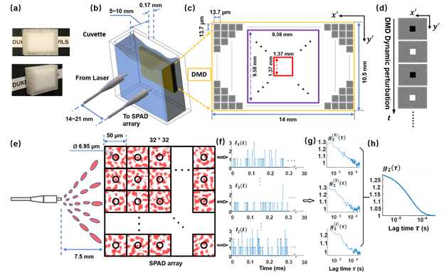
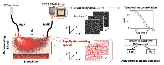
DCS systems are typically implemented in a reflection geometry, where a source and a detector are placed a finite distance d apart and detected light is assumed to travel through a “banana-shaped” point-spread function (PSF) that describes the light’s most probable path through scattering tissue. However, due to the forward-scattering nature of a biological tissue, most photons do not reach a detector in standard DCS measurement geometries, especially when the source and detector are place a large distance apart to probe deep events. We alleviate the problem with parallelized detection strategy. Since the optical modes emerging from the tissue are nearly mutually incoherent (i.e., decorrelating independently), detecting N fluctuating speckle grains simultaneously with multiple independent detectors bring a ![]() gain in the signal-to-noise ratio (SNR). We use a commercial SPAD camera containing 1024 independent detection channels to achieve detection. To quantitatively demonstrate the sensitivity and temporal resolution enhancements of our setup, we also design a novel phantom that consists of a digital micromirror device (DMD) placed directly behind a rapidly decorrelating tissue-mimicking phantom. The figure above shows the phantom configuration (a-d), the schematic layout of the distal end of the detection fiber and the SPAD array (e), and our data processing flow (f-h). Specifically, (a) Images of tissue phantom consisting of polystyrene microsphere-in-water suspension in a customized cuvette; (b) DMD phantom setup with DMD placed immediately behind tissue phantom. The distance between the centers of the illumination fiber and the detection fiber
gain in the signal-to-noise ratio (SNR). We use a commercial SPAD camera containing 1024 independent detection channels to achieve detection. To quantitatively demonstrate the sensitivity and temporal resolution enhancements of our setup, we also design a novel phantom that consists of a digital micromirror device (DMD) placed directly behind a rapidly decorrelating tissue-mimicking phantom. The figure above shows the phantom configuration (a-d), the schematic layout of the distal end of the detection fiber and the SPAD array (e), and our data processing flow (f-h). Specifically, (a) Images of tissue phantom consisting of polystyrene microsphere-in-water suspension in a customized cuvette; (b) DMD phantom setup with DMD placed immediately behind tissue phantom. The distance between the centers of the illumination fiber and the detection fiber ![]() was set to be approximately twice the cuvette thickness; (c) DMD panel. Square colored boxes represent different perturbation areas, varying from 1.37 × 1.37 mm2 to 9.58 × 9.58 mm2; (d) Example dynamic variation patterns, where pixels in middle square area switch between ‘on’ and ‘off’ states at a rate of multiple kHz (corresponding to the square color box in (c)), while the peripheral area is a constant random pattern; (e) Schematic layout of the 32 × 32 SPAD array illustrated with representative detected speckle patterns. The average speckle size at the SPAD array was tuned by adjusting detection fiber distance to approximately match the SPAD pixel active area (black circle). (f) Representative raw intensity measurements,
was set to be approximately twice the cuvette thickness; (c) DMD panel. Square colored boxes represent different perturbation areas, varying from 1.37 × 1.37 mm2 to 9.58 × 9.58 mm2; (d) Example dynamic variation patterns, where pixels in middle square area switch between ‘on’ and ‘off’ states at a rate of multiple kHz (corresponding to the square color box in (c)), while the peripheral area is a constant random pattern; (e) Schematic layout of the 32 × 32 SPAD array illustrated with representative detected speckle patterns. The average speckle size at the SPAD array was tuned by adjusting detection fiber distance to approximately match the SPAD pixel active area (black circle). (f) Representative raw intensity measurements, ![]() , from each SPAD pixel with a temporal resolution of 3 μs. (g) Corresponding intensity autocorrelation curves of each SPAD pixel,
, from each SPAD pixel with a temporal resolution of 3 μs. (g) Corresponding intensity autocorrelation curves of each SPAD pixel, ![]() , integrated over 30 ms, and (h) The final averaged autocorrelation curve
, integrated over 30 ms, and (h) The final averaged autocorrelation curve ![]() using all 1024 SPADs.
using all 1024 SPADs.
Results
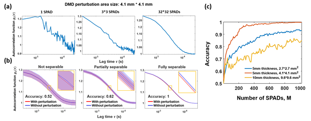
Fig. 4 – Demonstration of increased sensitivity to embedded perturbations with an increased number of SPADs. (a) Autocorrelation curves calculated using 1, 9 (3 × 3) and all 1024 (32 × 32) SPADs respectively, with an autocorrelation curve rate (![]() ) of 30 ms and a 4.1 × 4.1 mm2 DMD perturbation area; (b) Autocorrelation curve separability and corresponding perturbation detection accuracy using 1, 9 and 1024 SPADs. Banded curves represent the mean ± standard deviation (SD) of 420 averaged autocorrelations, where red curve is measurement with perturbation, and blue curve is measurement without perturbation; (c) Perturbation detection accuracy increases with a larger number of SPADs for three example setup configurations: 5 mm phantom thickness and 2.7 × 2.7 mm2 perturbation area (blue), 5 mm phantom thickness and 4.1 × 4.1 mm2 perturbation area (red), and 10 mm phantom thickness and 9.6 × 9.6 mm2 perturbation area (yellow).
) of 30 ms and a 4.1 × 4.1 mm2 DMD perturbation area; (b) Autocorrelation curve separability and corresponding perturbation detection accuracy using 1, 9 and 1024 SPADs. Banded curves represent the mean ± standard deviation (SD) of 420 averaged autocorrelations, where red curve is measurement with perturbation, and blue curve is measurement without perturbation; (c) Perturbation detection accuracy increases with a larger number of SPADs for three example setup configurations: 5 mm phantom thickness and 2.7 × 2.7 mm2 perturbation area (blue), 5 mm phantom thickness and 4.1 × 4.1 mm2 perturbation area (red), and 10 mm phantom thickness and 9.6 × 9.6 mm2 perturbation area (yellow).
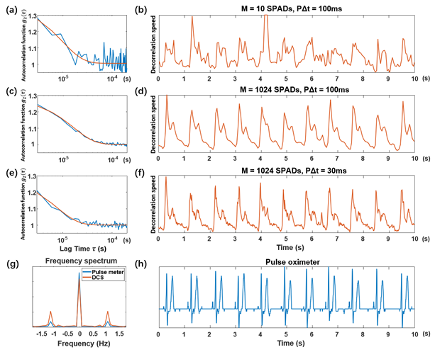
Fig. 8 – Human forehead pulse measurement results. Representative autocorrelation curves (blue) and their best exponential function fit (red) are at left (a, c, e). At right are associated DCS pulse measurements over 10 s (b, d, f), which are represented by the plot of normalized decorrelation speed, extracted from autocorrelation curves after exponential fitting. (a-b) Using M = 10 SPADs and an autocorrelation curve rate = 100 ms, (c-d) M = 1024 SPADs and an autocorrelation curve rate of = 100 ms, and (e-f) M = 1024 SPADs and an autocorrelation curve rate, = 30 ms. (g) The Fourier transform of the DCS pulse signal (f) and the pulse signal acquired using a commercial pulse meter (h).
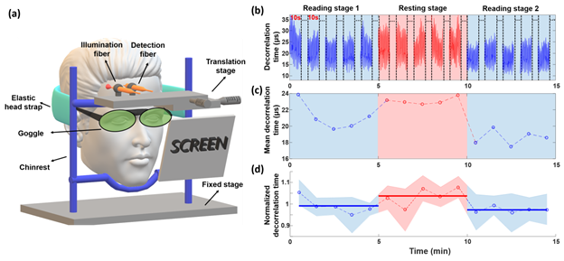
FIG. 9. The experimental setup and results of the human prefrontal cortex activation test. (a) The schematic diagram of the experimental setup. (b) The plot of the decorrelation time (td) values over the 15 min test including two reading stages and one intermediate rest stage, where 10 s of the signal is collected every minute. (c) The plot of mean decorrelation time corresponding to (b). Each mean decorrelation time value is obtained by averaging all the decorrelation time values within the corresponding 10 s window. (d) Mean ± SD results of the mean decorrelation time of 4 subjects calculated after dividing the data of each subject by the average decorrelation value of their respective measurement sequence. Solid horizontal lines represent the average of the five normalized decorrelation times in each stage.
Code and data
We have open-sourced the code and datasets necessary to reproduce the experimental results figures in our paper (Figs. 3-9):
Code: https://github.com/minor-planet/parallelized-DCS
Datasets: https://figshare.com/articles/dataset/Fast_and_sensitive_diffuse_correlation_spectroscopy_with_highly_parallelized_single_photon_detection/14067710